]— title: “WDI 2022 Exploratory Data Analysis” author: “Saahil Mardhekar” date: “2026-02-25” format: html: toc: true number-sections: true code-fold: true pdf: toc: true number-sections: true execute: echo: false warning: false message: false bibliography: references.bib crossref: true —

Data Source

This report analyzes 2022 country-level data from the World Development Indicators dataset published by the World Bank [@worldbank_wdi].

Load Data

import pandas as pd
import matplotlib.pyplot as plt

df = pd.read_csv("data/wdi.csv")
df.shape

(217, 14)

df.head()

	country	inflation_rate	exports_gdp_share	gdp_growth_rate	gdp_per_capita	adult_literacy_rate	primary_school_enrolment_rate	education_expenditure_gdp_share	measles_immunisation_rate	health_expenditure_gdp_share	income_inequality	unemployment_rate	life_expectancy	total_population
0	Afghanistan	NaN	18.380042	-6.240172	352.603733	NaN	NaN	NaN	68.0	NaN	NaN	14.100	62.879	41128771.0
1	Albania	6.725203	37.395422	4.856402	6810.114041	98.5	95.606712	2.74931	86.0	NaN	NaN	11.588	76.833	2777689.0
2	Algeria	9.265516	31.446856	3.600000	5023.252932	NaN	108.343933	NaN	79.0	NaN	NaN	12.437	77.129	44903225.0
3	American Samoa	NaN	46.957520	1.735016	19673.390102	NaN	NaN	NaN	NaN	NaN	NaN	NaN	NaN	44273.0
4	Andorra	NaN	NaN	9.563798	42350.697069	NaN	90.147346	2.66623	98.0	NaN	NaN	NaN	NaN	79824.0

Missing Data Overview

df.isna().sum().sort_values(ascending=False)

health_expenditure_gdp_share       197
income_inequality                  189
adult_literacy_rate                168
education_expenditure_gdp_share    112
primary_school_enrolment_rate      103
inflation_rate                      48
exports_gdp_share                   48
unemployment_rate                   31
measles_immunisation_rate           24
gdp_growth_rate                     15
gdp_per_capita                      14
life_expectancy                      8
country                              0
total_population                     0
dtype: int64

---

Indicator 1: GDP per Capita

df[["gdp_per_capita"]].describe()

Table 1: Summary statistics for GDP per capita (USD), WDI 2022.

	gdp_per_capita
count	203.000000
mean	20345.707649
std	31308.942225
min	259.025031
25%	2570.563284
50%	7587.588173
75%	25982.630050
max	240862.182448

df["gdp_per_capita"].dropna().plot(kind="hist", bins=30)
plt.title("GDP per Capita (2022)")
plt.xlabel("GDP per Capita (USD)")
plt.ylabel("Count")
plt.tight_layout()
plt.show()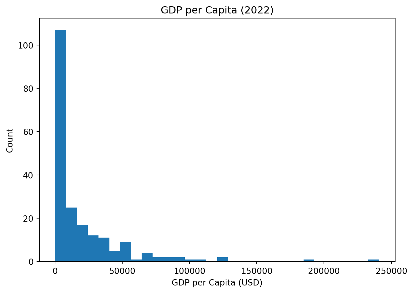

Figure 1: Distribution of GDP per capita (USD), WDI 2022. Source: World Bank WDI [@worldbank_wdi].

See Figure Figure 1 and Table Table 1.

---

Indicator 2: Life Expectancy

df[["life_expectancy"]].describe()

Table 2: Summary statistics for life expectancy (years), WDI 2022.

	life_expectancy
count	209.000000
mean	72.416519
std	7.713322
min	52.997000
25%	66.782000
50%	73.514634
75%	78.475000
max	85.377000

sub = df[["gdp_per_capita", "life_expectancy"]].dropna()

plt.scatter(sub["gdp_per_capita"], sub["life_expectancy"])
plt.title("Life Expectancy vs GDP per Capita (2022)")
plt.xlabel("GDP per Capita (USD)")
plt.ylabel("Life Expectancy (years)")
plt.tight_layout()
plt.show()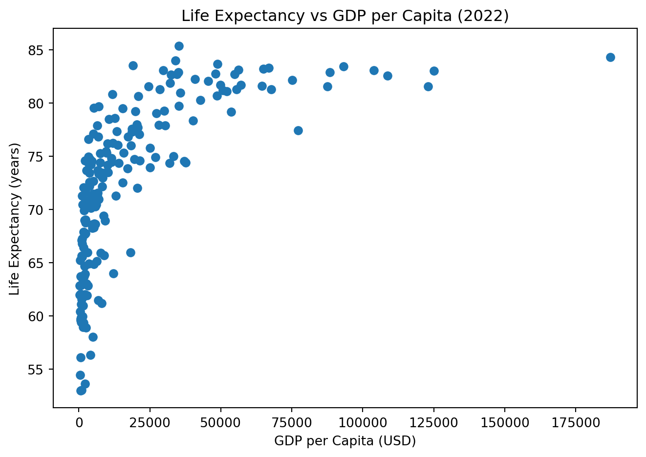

Figure 2: Life expectancy vs GDP per capita, WDI 2022. Source: World Bank WDI [@worldbank_wdi].

See Figure Figure 2 and Table Table 2.

---

Indicator 3: Unemployment Rate

df[["unemployment_rate"]].describe()

Table 3: Summary statistics for unemployment rate (%), WDI 2022.

	unemployment_rate
count	186.000000
mean	7.268661
std	5.827726
min	0.130000
25%	3.500750
50%	5.537500
75%	9.455250
max	37.852000

top_unemp = (
    df[["country", "unemployment_rate"]]
    .dropna()
    .sort_values("unemployment_rate", ascending=False)
    .head(15)
)

plt.bar(top_unemp["country"], top_unemp["unemployment_rate"])
plt.title("Top 15 Unemployment Rates (2022)")
plt.xlabel("Country")
plt.ylabel("Unemployment Rate (%)")
plt.xticks(rotation=60, ha="right")
plt.tight_layout()
plt.show()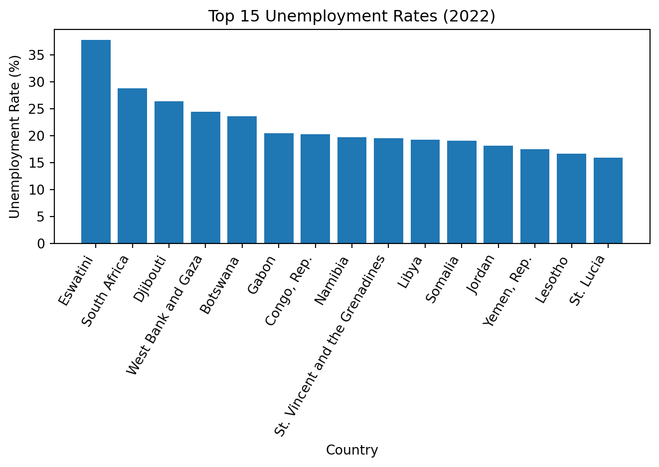

Figure 3: Top 15 countries by unemployment rate (%), WDI 2022. Source: World Bank WDI [@worldbank_wdi].

See Figure Figure 3 and Table Table 3.

---

Combined Key Statistics

key = df[["gdp_per_capita", "life_expectancy", "unemployment_rate"]]

summary = pd.DataFrame({
    "count": key.count(),
    "mean": key.mean(),
    "median": key.median(),
    "std": key.std(),
    "min": key.min(),
    "max": key.max()
})

summary

Table 4: Key statistics for GDP per capita, life expectancy, and unemployment rate, WDI 2022.

	count	mean	median	std	min	max
gdp_per_capita	203	20345.707649	7587.588173	31308.942225	259.025031	240862.182448
life_expectancy	209	72.416519	73.514634	7.713322	52.997000	85.377000
unemployment_rate	186	7.268661	5.537500	5.827726	0.130000	37.852000

See Table Table 4.

---

Interpretation

GDP per capita shows a strongly right-skewed distribution, indicating that a small number of countries have very high income levels relative to the majority. Life expectancy generally increases with GDP per capita, suggesting a positive association between income and health outcomes. Unemployment rates vary widely across countries and do not display a simple linear pattern with GDP per capita. These findings are based on available 2022 data from the World Development Indicators dataset [@worldbank_wdi].

References